Code
install.packages(here::here("data/microarray/org.Psativum1c.eg.db"), repos = NULL, type = "source")Install from a local folder
install.packages(here::here("data/microarray/org.Psativum1c.eg.db"), repos = NULL, type = "source")# pkg
library(tidyverse)
library(org.Psativum1c.eg.db) # if not working install it
library(clusterProfiler)
library(readxl)
library(GO.db)
library(AnnotationDbi)
library(ggnewscale) # to have two scale_fill
# src
source(here::here("src/function/fig_export.R")) # This function saves a given plot (plot_x) as both a PDF and a high-resolution PNG file at specified dimensions.
source(here::here("src/function/upsetplot_condition_merge_sign.R")) # function "create_presence_matrix" and "upsetplot_condition_merge_sign"
# cosmetics
water_pallet=read_excel(here::here("data/color_palette.xlsm")) %>%
filter(set == "water_condition") %>%
dplyr::select(color, treatment) %>%
pull(color) %>%
setNames(read_excel(here::here("data/color_palette.xlsm")) %>%
filter(set == "water_condition") %>%
pull(treatment)
)
my_color_palette <- read_excel(here::here("data/color_palette.xlsm"))# Get GO and gene description for all gene loci
keytypes(org.Psativum1c.eg.db)
all_genes <- keys(x=org.Psativum1c.eg.db, keytype = "GID")
all_GO <- AnnotationDbi::select(x = org.Psativum1c.eg.db, keys = all_genes, columns =c("GO","ONTOLOGY") , keytype = "GID")
# Select Biological Processes
all_GO_BP <- all_GO[all_GO$ONTOLOGY == "BP",] %>%
na.omit() %>%
dplyr::select("GO", "GID") %>%
dplyr::rename(go_id = GO,
gene_id = GID)
# collect data and add Psat to PsCAM
load(file = here::here("data/microarray/output/ratio_stats_microarray_root_nodule_FABER.RData"))
df_info_gene <- list_ratio_stats_global %>%
map("id_probe") %>%
compact() %>%
unlist(use.names = FALSE) %>%
unique() %>%
as.data.frame() %>%
rename(PsCam = ".") %>%
left_join(.,read_excel(here::here("data/microarray/Resultats_12plex-PEA-2013-03_NODULES_mod_281014.xlsx"), sheet = "Pscam_to_Psat_v1c_mrna_besthit-", col_names = T), by = "PsCam")
write_csv(x = df_info_gene, file = here::here("data/microarray/output/info_gene.csv"))
write_csv(x = all_GO_BP, file = here::here("data/microarray/output/all_GO_BP.csv"))load(file = here::here("data/microarray/output/upset_result_condition_sign_all.RData"))
df_info_gene <- read_csv(file = here::here("data/microarray/output/info_gene.csv"), show_col_types = FALSE)
all_GO_BP <- read_csv(file = here::here("data/microarray/output/all_GO_BP.csv"), show_col_types = FALSE)
cluster_info <- rbind(purrr::imap_dfr(lt_down, ~ tibble(PsCam = .x, comparison = .y)) %>%
mutate(cluster = paste0("(Down) ", comparison)),
purrr::imap_dfr(lt_up, ~ tibble(PsCam = .x, comparison = .y)) %>%
mutate(cluster = paste0("(Up) ", comparison))
) %>% full_join(., df_info_gene, by = "PsCam") %>%
mutate(ID = Psat) %>%
drop_na(comparison, ID)
cluster_info %>% filter(PsCam == "PsCam042688")
# Add a filter on cov ? or id ?
# Run GO enrichment analysis with by cluster
#-------------------------------------------
# Initialize an empty list to store results for each cluster
all_results <- list()
# Loop through each unique cluster in `cluster_info`
for (i in unique(cluster_info$cluster)) {
# Extract the gene list for the current cluster
gene_list <- cluster_info %>% filter(cluster == i) %>% pull(ID)
# Perform enrichment analysis for the current cluster
enrichment_results <- enricher(gene = gene_list,
TERM2GENE = all_GO_BP,
pvalueCutoff = 0.05,
pAdjustMethod = "BH",
minGSSize = 10,
maxGSSize = 500)
# Convert the enrichment results to a data frame and add a column for the cluster ID
if (!is.null(enrichment_results) && nrow(as.data.frame(enrichment_results)) > 0) { # Check if there are results for the current cluster
enrichment_df <- as.data.frame(enrichment_results)
enrichment_df$cluster <- i # Add the cluster ID to the results
all_results[[as.character(i)]] <- enrichment_df # Store in the list
}
}
# Combine all cluster results into a single data frame
combined_results <- bind_rows(all_results)
# Get the GO description
go_terms <- keys(GO.db)
go_descriptions <- Term(go_terms)
go_table <- data.frame(GO_Term = go_terms, Description_GO = go_descriptions)
names(go_table)[1] <- "ID"
combined_results <- left_join(combined_results, go_table, by = "ID")
combined_results %>% filter(str_detect(geneID, "Psat3g185920"))
cluster_info %>% filter(PsCam == "PsCam042688")
write_csv(x = combined_results, file = here::here(paste0("data/microarray/output/GO_BP_deregulated_genes.csv")))# parameter
combined_results <- read_csv(file = here::here(paste0("data/microarray/output/GO_BP_deregulated_genes.csv")), show_col_types = FALSE)
combined_results.top <- combined_results %>%
dplyr::group_by(cluster) %>%
top_n(-10, wt = p.adjust) %>%
arrange(cluster, p.adjust)
# Define the list of selected significant GO terms
Signif_GO <- unique(combined_results.top$Description)
# Filter results based on this list
Cluster_selected_GO <- filter(combined_results, ID %in% Signif_GO)
# Ensure GeneRatio and BgRatio are character columns
Cluster_selected_GO_2 <- Cluster_selected_GO
str(Cluster_selected_GO_2)
Cluster_selected_GO_2$GeneRatio <- as.character(Cluster_selected_GO_2$GeneRatio)
Cluster_selected_GO_2$BgRatio <- as.character(Cluster_selected_GO_2$BgRatio)
# Calculate the fold enrichment
Cluster_selected_GO_2$FoldEnrichment <- with(Cluster_selected_GO_2,
(sapply(strsplit(GeneRatio, "/"), function(x) as.numeric(x[1]) / as.numeric(x[2]))) /
(sapply(strsplit(BgRatio, "/"), function(x) as.numeric(x[1]) / as.numeric(x[2]))))
# Calculate the -log10(pvalue)
Cluster_selected_GO_2$'|-log10(Pval)|' <- -(log10(Cluster_selected_GO_2$p.adjust))
# Ensure that `Term` column has factor levels including all possible terms
Cluster_selected_GO_2$Description_GO <- factor(Cluster_selected_GO_2$Description_GO, levels = unique(Cluster_selected_GO_2$Description_GO))
# Now, create a data frame with all combinations of `Term` and `filename`
all_combinations <- expand.grid(Description_GO = levels(Cluster_selected_GO_2$Description_GO), cluster = unique(cluster_info$cluster))
# Merge this with your original data to fill missing combinations
Cluster_selected_GO_filled <- merge(all_combinations, Cluster_selected_GO_2, by = c("Description_GO", "cluster"), all.x = TRUE) %>%
mutate(cluster = factor(cluster,
levels = unique(cluster)),
comparison = str_trim(str_remove(cluster, "\\s*\\(.*?\\)")),
sign = str_extract(cluster, "(?<=\\().*?(?=\\))")
) %>%
mutate(comparison = forcats::fct_relevel(comparison, "Root_WW_D vs Root_WW_C", "Root_WS_C vs Root_WW_C", "Root_WS_D vs Root_WS_C", "Root_WS_D vs Root_WW_D",
"Nodule_WW_D vs Nodule_WW_C", "Nodule_WS_C vs Nodule_WW_C", "Nodule_WS_D vs Nodule_WS_C", "Nodule_WS_D vs Nodule_WW_D"))
# creation of the color (same as upsetplot)
# vector_color <- c(lighten(as.character(sulfate_pallet[1]), amount = -.2),
# lighten(as.character(sulfate_pallet[1]), amount = .5),
# lighten(as.character(sulfate_pallet[2]), amount = -.2),
# lighten(as.character(sulfate_pallet[2]), amount = .3),
# "#9381FF"
# )
#vector_color <- c("#067B5B", "#6AD6AD", "#B87100", "#FFAC5C", "#9381FF", "#067B5B", "#6AD6AD", "#B87100", "#FFAC5C", "#9381FF")
# Plot the enrichment by GO
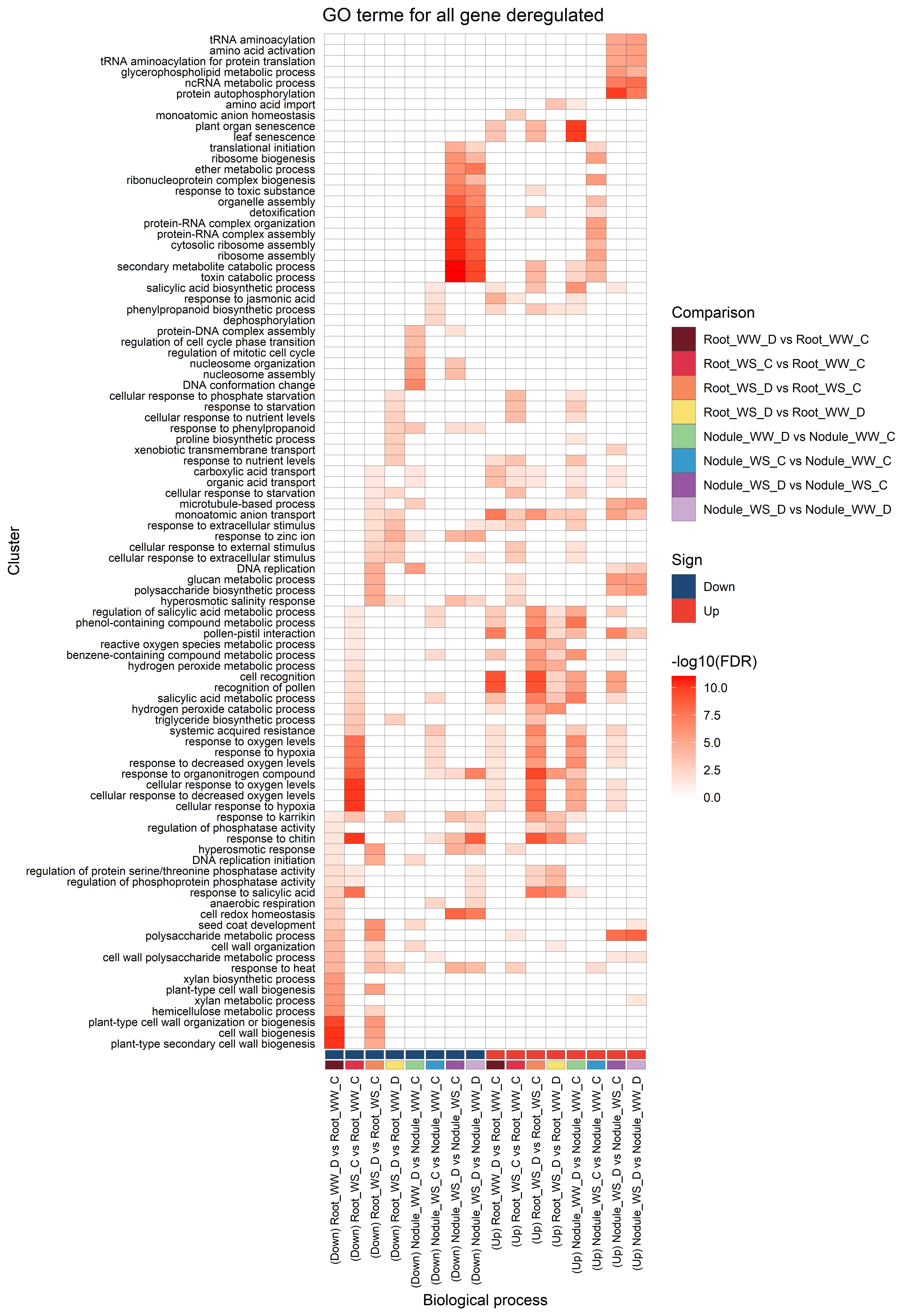
px <- ggplot(Cluster_selected_GO_filled, aes(x = cluster, y = Description_GO, fill = `|-log10(Pval)|`)) +
geom_tile(color = "black") +
scale_fill_gradient2(low = "white", high = "red", na.value = "white", limits = c(0, NA)) +
theme_minimal() +
theme(axis.text = element_text(size = 8, colour = "black"),
axis.text.x = element_text(angle = 90, vjust = 0.5, hjust = 1),
panel.grid.major = element_blank(),
plot.background = element_rect(fill = "white", colour = "white")) +
labs(fill = "-log10(FDR)",
x= "Biological process",
y = "Cluster",
title = "GO terme for all gene deregulated") +
#scale_size_manual(values = c(dot = 2, no_dot = NA), guide = "none")+
new_scale_fill() +
scale_fill_manual(
values = c("#6f1926", "#de324c", "#f4895f", "#f8e16f", "#95cf92", "#369acc", "#9656a2", "#cbabd1"),
name = "Comparison"
) +
geom_tile(
aes(
x = cluster,
y = -1, # If you truly want it at a negative y-value,
# ensure your y-scale is continuous or can handle this
fill = comparison,
width = 0.90,
height = 0.80
),
data = Cluster_selected_GO_filled,
color = "black",
alpha = 1,
inherit.aes = FALSE
)+
new_scale_fill() +
scale_fill_manual(
values = c('Down' = "#1d4877", 'Up' = "#ee3e32"),
name = "Sign"
) +
geom_tile(
aes(
x = cluster,
y = -0.05, # If you truly want it at a negative y-value,
# ensure your y-scale is continuous or can handle this
fill = sign,
width = 0.90,
height = 0.80
),
data = Cluster_selected_GO_filled,
color = "black",
alpha = 1,
inherit.aes = FALSE
) ; px
# export
fig_export(path = "report/microarray/plot/GO/GO_all_absolute", plot_x = px, height_i = 13, width_i = 9, res = 600)